This analysis tests two competing capacity investment strategies — one targeting the obvious bottleneck, one targeting the actual constraint — to determine which is worth the money.
Setup
A manufacturing job shop runs 8 jobs across 6 machines (Table Saw, CNC Router, Sander, Drill Press, Assembly Bench, Finishing Station). The system operates in weekly production cycles with fixed routing and machine constraints.
| Job | Ops | Deadline | Baseline |
|---|---|---|---|
| Nightstand (×2) | 5 | 60h | On time |
| Desk | 6 | 80h | On time |
| Bookshelf | 7 | 90h | On time |
| Coffee Table | 6 | 75h | Late +17h |
| Chair Set (×4) | 8 | 110h | Late +16h |
| Dining Table | 8 | 130h | Late +13h |
| Cabinet | 9 | 140h | Late +29h |
| Wardrobe | 9 | 160h | Late +46h |
58 operations total, each with a specific machine, duration, and precedence constraints.
We build the production schedule as a constraint optimization problem using MiniZinc + OR-Tools CP-SAT, minimizing total tardiness. Even with an optimal schedule, 5 of 8 jobs are late with 121 hours of tardiness. This isn’t a planning problem; the tardiness is structural. It can’t be scheduled away, it requires a capacity intervention, and we use the baseline schedule to quantify which intervention is worth the money.
Choosing the Interventions
The baseline analysis surfaces two distinct bottleneck profiles:
| Machine | Utilisation | Critical Ops | Profile |
|---|---|---|---|
| Table Saw | 71% | 22 of 58 | Critical chokepoint, dominates the critical path |
| Sander | 36% | 1 of 58 | Amplifier, low utilisation but affects every tardy job |
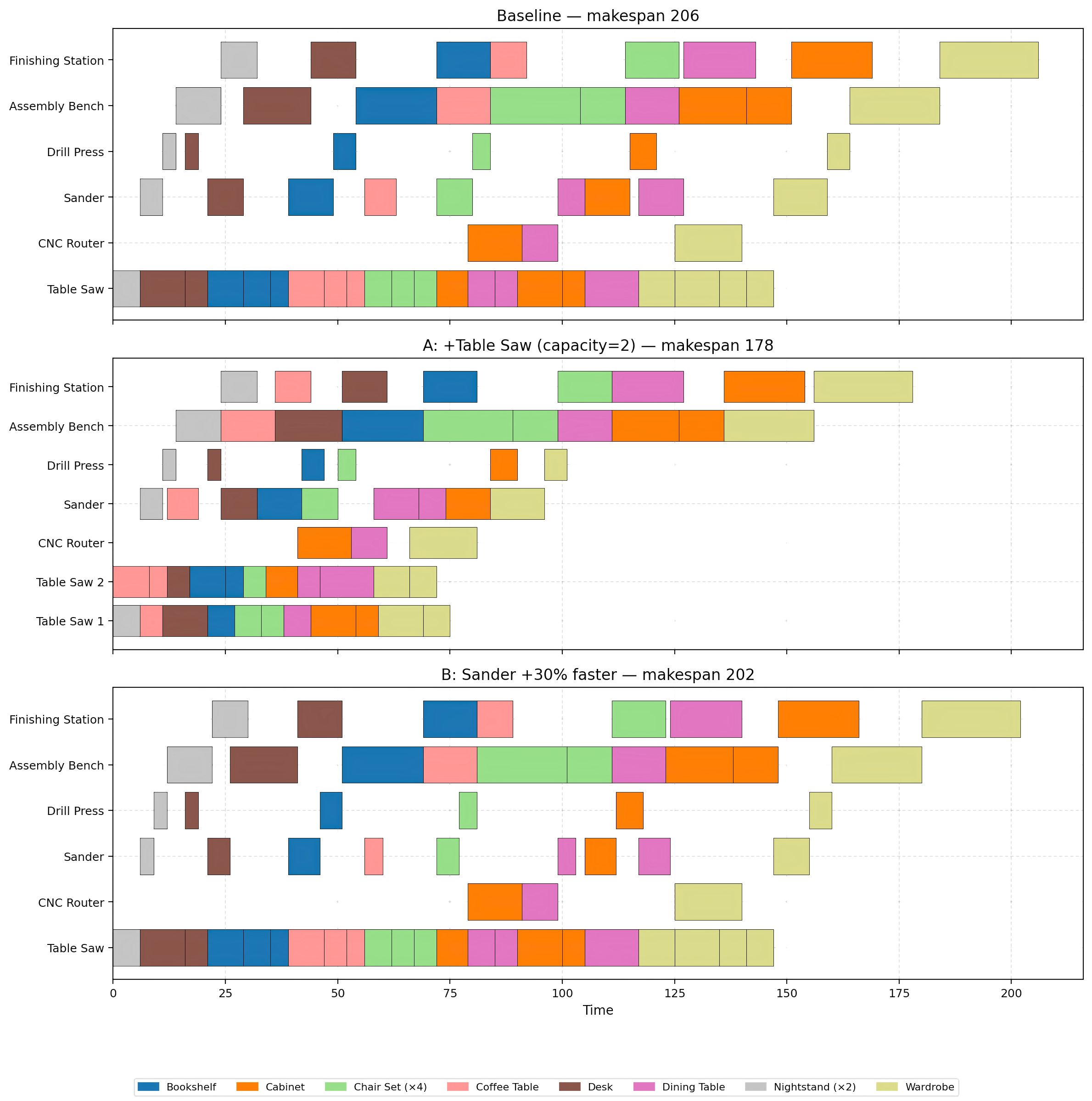
A naive bottleneck analysis would target the Sander: it’s cheap to improve (low utilisation means a small speedup unlocks downstream slack) and it sits on the routing of all five late jobs. But “on the routing” is not the same as “on the critical path” — the Sander only constrains one operation in the entire schedule. Touching every late job makes it look influential; having only one critical op means it isn’t the thing holding those jobs up.
The Table Saw is already heavily loaded, adding capacity looks expensive. But it sits on the critical path for nearly half the operations. If it’s the true bottleneck, adding capacity there could cascade improvements that no amount of Sander tuning can match.
We test both:
- Experiment A: Add a second Table Saw (CAPEX $45,000)
- Experiment B: Improve Sander throughput by 30% (CAPEX $8,000)
Executive Summary
- The Table Saw carried 22 of 58 operations on the critical path. The Sander touched every late job but had only 1 critical operation. Touching everything doesn't make something a bottleneck.
- Adding a second Table Saw reduced tardiness by 73% ($17,600 per production run). A 30% Sander improvement reduced it by just 13%. Both paid back in ~2.5 runs.
- The Table Saw delivered 5.5× higher savings per run because it removed a binding constraint on the critical path — despite higher upfront cost.
- A naive bottleneck analysis would have targeted the Sander. Counterfactual simulation showed the Table Saw was the real constraint. Utilization alone is not a reliable guide for capacity investment decisions.
Results
KPI Comparison
Impact of capacity interventions on throughput, tardiness, and schedule stability.
| KPI | Baseline | +Table Saw | Δ A | Sander +30% | Δ B |
|---|---|---|---|---|---|
| Makespan | 206h | 178h | -13.6% | 202h | -1.9% |
| Max Tardiness | 46h | 18h | -60.9% | 42h | -8.7% |
| Avg Tardiness | 15.1h | 4.1h | -72.7% | 13.1h | -13.2% |
| Late Jobs | 5 | 3 | -2 | 5 | 0 |
| Late Job Ratio | 62.5% | 37.5% | -25.0pp | 62.5% | 0 |
| Deadline-Norm Tardiness | 96.7% | 22.2% | -74.5pp | 83% | -13.7pp |
| Load-Norm Tardiness | 22.7% | 6.2% | -16.5pp | 20.8% | -2.0pp |
| Critical Op Ratio | 44.8% | 25.9% | -19.0pp | 44.8% | 0 |
Machine Schedules (Side-by-Side)
Per-Job Tardiness
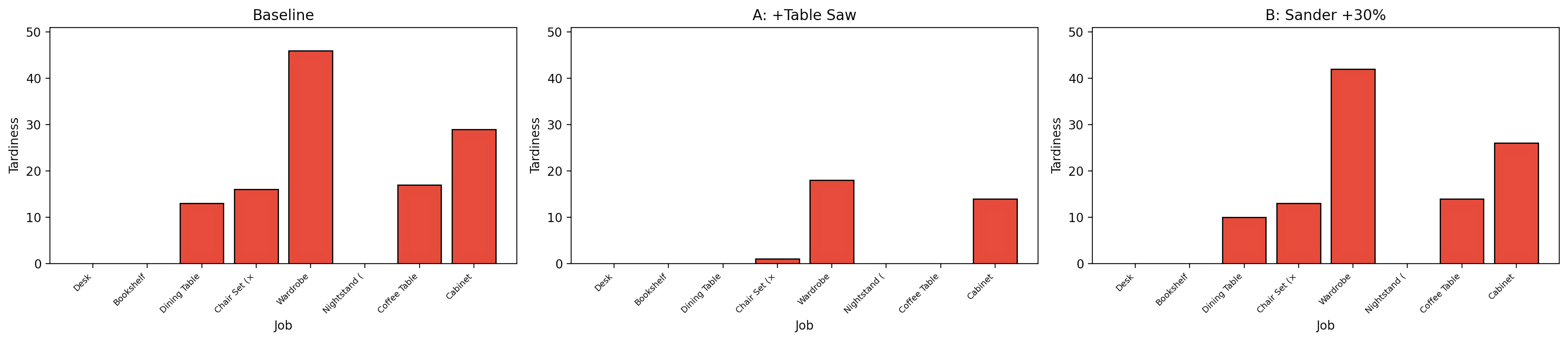
Cost Analysis
Assumptions:
- Tardiness penalty: $200 per hour of tardiness per job set
- Runs per week: 1
Baseline tardiness cost per job set: $24,200 (121 hours)
Experiment A: Add a second Table Saw (CAPEX $45,000)
- Tardiness savings per job set: $17,600 (88 hours × $200/hour)
- Payback period: 2.6 weeks (2.6 runs)
- First-year net savings: $870,200 (ROI: +1,934%)
Experiment B: Improve Sander throughput 30% (CAPEX $8,000)
- Tardiness savings per job set: $3,200 (16 hours × $200/hour)
- Payback period: 2.5 weeks (2.5 runs)
- First-year net savings: $158,400 (ROI: +1,980%)
Recommendation
| Tardiness (h) | Reduction | Savings/run | Payback | 1st-year net | |
|---|---|---|---|---|---|
| +Table Saw | 33h | 73% | $17,600 | 2.6 runs | $870,200 |
| Sander +30% | 105h | 13% | $3,200 | 2.5 runs | $158,400 |
Both interventions pay back in ~2.5 runs. The difference is magnitude: the second Table Saw delivers 73% tardiness reduction ($17,600 saved per run) vs. 13% ($3,200 per run) for the Sander upgrade. Although both investments recover their cost in roughly the same number of production runs, the Table Saw delivers 5.5× higher savings per run by removing a binding constraint on the critical path. The Sander, despite its system-wide presence, does not materially constrain the schedule.
Methodology
This follows the same workflow used in operational decision studies:
- Build a feasible production schedule for the 8-job, 6-machine shop using MiniZinc + OR-Tools CP-SAT, minimising total tardiness.
- Identify critical resources from the baseline — here, the Table Saw (dominant critical path) and the Sander (wide routing footprint but weak constraint).
- Model two alternative capacity interventions: a second Table Saw and a 30% Sander throughput improvement, each with CAPEX cost.
- Re-optimise the schedule under each scenario and collect the same KPIs (makespan, tardiness distribution, critical op ratio).
- Compare operational metrics and economic outcomes to decide which investment is worth the money.
The objective is not only to produce a schedule, but to quantify the expected impact of operational changes before capital is committed — evaluated through throughput, lateness reduction, and economic impact.
Conclusion
Capacity decisions rarely align with utilisation or intuitive bottleneck signals. In this system, the Sander appeared influential due to its broad routing footprint, while the Table Saw — embedded in the critical path — governed overall system performance. The intuitive choice (cheaper, broader reach) underperforms. The counterintuitive choice (expensive, narrow focus) delivers 5.5× the savings. These differences only become visible under counterfactual simulation, where structural constraints are explicitly tested rather than inferred.